Alright, enough theoretical discussion! Let’s try out empirical generalized information (EGI) on a machine learning problem.

In this case, we construct an artificial problem of some complexity using logical formulas of Boolean variables. Each variable in the formula can either be true or false. The variables are combined with the logical operators NOT, OR, and AND. For example,

A AND B is only true if both A and B are true.

NOT C is only true if C is false.

D OR E is only false if both D and E are false.

Using these operators we connect a large number of variables and balance the expression so there is about a 50% chance of getting true or false by randomly assigning values to the variables. Doing this means that we have a problem that can be learned because it has a logical structure.

Imagine that Bob wants to buy a new vehicle. Sam wants to sell Bob a vehicle but he does not know what Bob wants. However, Sam does have a record of 1000s of vehicles that Bob is interested or not interested in, based on his browsing history.

Sam’s problem is that the 1000s of likes and dislikes need to be translated to a summary of Bob’s preferences. Fortunately, this is exactly the sort of problem we can represent with Boolean variables and solve using the decision tree algorithm.

For example, Bob has shown an interest in red sports cars, inexpensive black trucks, and blue golf carts. We can represent this set of preferences with eight boolean variables, using the following logic formula:

(RED and SPORTY and CAR)

or

(CHEAP and BLACK and TRUCK)

or

(BLUE and GOLF CART)

Sam, who cannot read Bob’s mind, must infer the formula from the 1000s of likes and dislikes. He notices that the logic of the preference formula can be described using a decision tree.

For instance, given a vehicle, we can follow a set of decision criteria to determine if Bob would like the vehicle. If the vehicle is red, then we check if it is sporty. If it is sporty, then we check if it is a car.

If so, then we know it is one of the types of vehicle that Bob likes. Thus Sam can model the preference formula as a decision tree, and use the likes and dislikes he has gathered from Bob to construct the tree.

To train the decision tree, Sam uses a standard machine learning metric called the Gini metric. The Gini metric is similar to entropy, but is often preferred in decision tree building because it results in more accurate trees. It works similarly to entropy, in that it is a measure of the number of choices and uncertainty. A greater number of choices means greater uncertainty. Fewer choices means more certainty. Thus, the model with the lowest Gini score provides the least uncertainty and best predictive accuracy on the training dataset.

However, as we’ve discussed previously, a high predictive accuracy on the training dataset does not automatically mean a model will have high predictive accuracy on new data; the decision tree may end up memorizing the training data, thus ‘cheating’ on the test. There are “rule of thumb” ways to prevent memorization, such as limiting the size of the decision tree. But we would like a more principled way to prevent memorization and guarantee generalization. So, for comparison, Sam uses the EGI metric to train another decision tree on the same data and compares it to the tree generated with the Gini metric.

To run the comparison test, Sam splits his dataset of Bob’s likes and dislikes into a training set and a holdout set. Sam trains the decision trees using both the the Gini metric and the EGI metric on the training set. He then checks the model’s accuracy on the holdout set.

However, this test by itself will not show Sam whether the models are generalizing. To really test whether the models are generalizing, Sam needs to add random noise to the training set. If the model generalizes, then as noise is added it will perform better than a model that does not generalize. Additionally, if the metric is good at avoiding meaningless information, then—as noise is added—the model size will shrink. So Sam runs a number of tests, each adding a greater amount of noise, until the training set is indistinguishable from random noise.

Now the moment we have been waiting for: We get to see Sam’s results. First, Sam shows us how the EGI and Gini models differ in model size as noise increases:

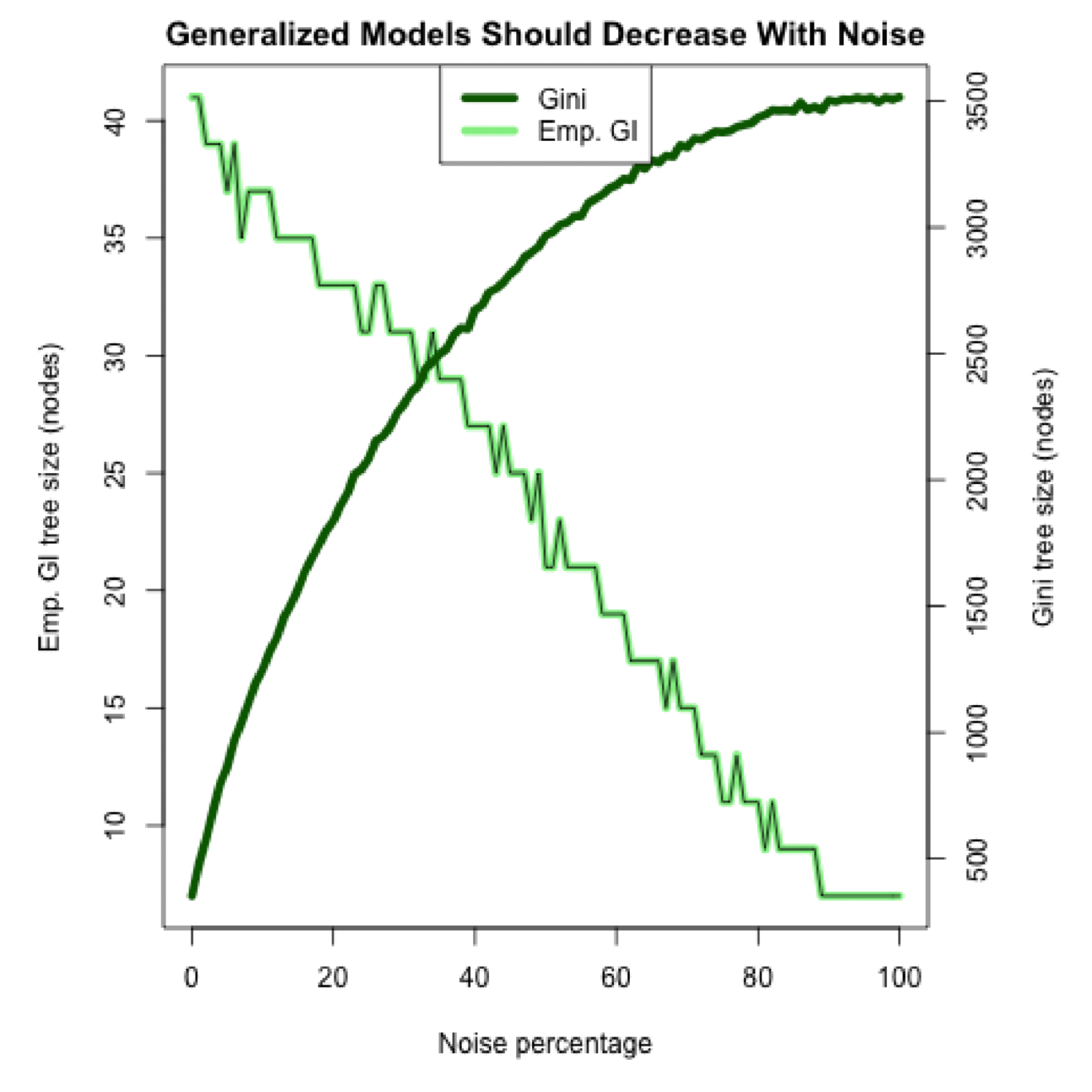
The difference is very clear. The model sizes vary inversely to each other as the noise increases, which is the expected outcome of a generalizing model compared with a model that does not generalize. However, this does not tell us whether EGI is in fact generalizing while Gini does not. For that, we will look at the second result graph that compares the raw accuracy of both models on the holdout set. If EGI does not generalize, then we will see the accuracy degrade proportional to the noise increase. On the other hand, if EGI does generalize, then accuracy will remain high even as noise is added. Here is Sam’s accuracy graph on the holdout set:

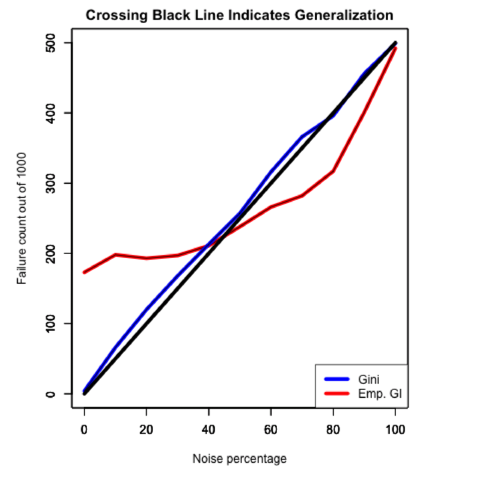
On the holdout accuracy graph we see a couple of interesting things. But the graph needs a bit of explanation. The important marker for generalization is the diagonal black line. It represents the expected amount a non-generalizing model can learn on the training data as noise is added to the training data. This means that if the model accuracy crosses onto the right side of the diagonal line then the model has successfully generalized. Thus, we see the EGI metric successfully causes the model to generalize.

However, this generalization ability comes at a cost. Because the metric penalizes large models, it is unable to learn from all the available information when there is no noise in the dataset. So, when there is only a small amount of noise in the training data, the Gini metric results in better accuracy on the holdout dataset. There is a way to get the best of both worlds, but that is a discussion for another time.

Back to Sam, what does Sam get out of this comparison of the Gini to the EGI metric? Sam has to think about Bob’s predilection for clicking likes and dislikes. Does Bob always click in line with his preference formula, or does he sometimes click counter to the preference formula? If there is no noise in Bob’s dataset, then Sam should use the Gini metric and extract everything he can from the dataset. Or, if Bob does add noise to the dataset after having read a car magazine and getting a brief liking for blue sedans and orange trucks, then Sam should use a metric like EGI that can generalize in the presence of noise.

Given that humans tend to add a bit of noise to their choices, Sam is benefited by having access to a generalization metric like EGI. Otherwise, Sam might accidentally select the hot pink Mini Cooper that Bob’s fifteen-year-old daughter was looking at while logged into his account.

Alright, now that Sam has his generalized model, how does he turn it into Bob’s preference formula? Sam simply collects all the leaves in the decision tree that strongly predict a like. Tracing the decisions from the root to each leaf gives the criteria for each kind of vehicle that Bob likes.

One final item of interest to note. In normal machine learning, we test whether our model is memorizing or generalizing with the holdout dataset. But, if we can measure our model’s generalization using just the training dataset, as is possible with EGI, then why have a holdout dataset? Good observation!

The holdout dataset is unnecessary if we can measure generalization. This means that Sam can use all of Bob’s clicks to train the model, resulting in an even more accurate representation of Bob’s preference formula. The ability to use all the data for training is one more practical benefit of being able to measure generalization.

In conclusion, the takeaway from this eight-part discussion and experiment is that, contrary to traditional Fisherian hypothesis testing, it is possible to create models after viewing the data and still quantify the generality of the model. The key principle that allows us to do this is the observation that, in order to generalize, the model needs to be independent from the data.

One way of guaranteeing this independence is measuring model size. There are only a few small models and thus it is highly unlikely for a small model to accurately predict a large number of events. Consequently, by calculating a tradeoff between the number of guesses, the accuracy of the guesses, and the size of the model, we arrive at the principled EGI metric that can quantify whether our model has generalized.

To summarize, we now live in an era of post-Fisherian hypothesis testing.

Machine learning isn’t difficult; just different. A few simple principles open many doors. Here are the previous instalments in the series:

Part 1 in this series by Eric Holloway is The challenge of teaching machines to generalize. Teaching students simply to pass tests provides a good illustration of the problems. We want the machine learning algorithms to learn general principles from the data we provide and not merely little tricks and nonessential features that score high but ignore problems.

Part 2: Supervised Learning. Let’s start with the most common type of machine learning, distinguishing between something simple, like big and small.

Part 3: Don’t snoop on your data. You risk using a feature for prediction that is common to the dataset, but not to the problem you are studying

Part 4. Occam’s Razor Can Shave Away Data Snooping. The greater an object’s information content, the lower its probability. If there is only a small probability that our model is mistaken with the data we have, there is a very small probability that our model will be mistaken with data we do not have.

Part 5: Machine Learning: Using Occam’s Razor to generalize. A simple thought experiment shows us how. This approach is contrary to Fisher’s method where we formulate all theories before encountering the data. We came up with the model after we saw the cards we drew.

Part 6: Machine Learning: Trees can solve murders. Decision trees increase our chance at a right answer. We can see how that works in a mystery board game like Clue. Entropy is a concept in information theory that characterizes the number of choices available when a probability distribution is involved. Understanding how it works helps us make better guesses.

Part 7: Machine learning: Harnessing the power of Empirical Generalized Information (EGI). We can calculate a probability bound from entropy. Entropy also happens to be an upper bound on the binomial distribution. We want our calculation to demonstrate the notion that if we have high accuracy and a small model, then we have high confidence of generalizing. Intuitively, then, we add the model size to the accuracy and subtract this quantity from the entropy of having absolutely no information about the problem.

For more general background on machine learning:

Part 1: Navigating the machine learning landscape. To choose the right type of machine learning model for your project, you need to answer a few specific questions (Jonathan Bartlett)

Part 2: Navigating the machine learning landscape — supervised classifiers Supervised classifiers can sort items like posts to a discussion group or medical images, using one of many algorithms developed for the purpose. (Jonathan Bartlett)